| |
The MEG Replication
Project by hyiq.org
Please Note: The MEG
is a Patented Device. hyiq.org has been granted permission for this
Replication by The MEG's Inventors.
|
Tom
Bearden "One build-up has produced up to 100 times more
power than was input"
A basic
idea on how The MEG Works.
The MEG has some history. Although patented in 2002 by Thomas
E. Bearden, Ph.D. James C. Hayes, Ph.D. James L. Kenny,
Ph.D. Kenneth D. Moore, B.S. Stephen L. Patrick, B.S. The
MEG has operational characteristics of many other devices
throughout History. Some may disagree with my opinion but
that's all this page is about, my opinion on how the MEG
Works.
Simply put, The MEG is See-Sawing Electromagnetic Flux from
the Permanent Magnet from side to side of the MetGlas Cores.
As the name suggests The MEG is a Generator, just a stationary
one. The actual EMF Generated in the Output Coils is induced
in a slightly different manner than the EMF Generated in
a Conventional Generator, or at least how current theory
says EMF is Generated in Generators. We must remember the
great Michael Faraday only said, we only have to have a
Flux move in relation to the Conductor to generate an EMF
in the conductor.
A Magnet's Flux is made up of several things (called vectors
and potentials), we look at these forces in a manner where
we can define these forces in a manner similar to a River.
This is similar to Electricity, Flow and Current. Flow can
be the amount of water flowing in a River, or Volts in a
Electrical Circuit and, Current, how much force or power
the Flow is travelling at, similar to the Current in an
Electrical Circuit. These differences are defined as the
H field, (Current or strength) and the B Field, (Flow or
volume). Looking at Magnetic, or Electromagnetic Flux is
made simple when viewed in these terms.
To move Magnetic or Electromagnetic Flux requires Force.
In the terms of a River, to stop the flow of a river we
must have a river flowing, equal in Flow and Current, flowing
in the opposite direction to the River we wish to stop.
Like in the Flux-Gate Magnetometers, it is very important
to look at The MEG in two halves. One half on one side and
the other half on the other side. Each side containing a
Power Coil and an Actuator Coil. The Power coil and Actuator
Coil on one side do not match up as a pair. In fact the
Power Coil on one side matches up with the Actuator Coil
on the opposing half of The MEG.
In an idle state, The MEG has equal Flux in each side of
the Core. The idea is that we want to create an imbalance
with our input.
In The MEG we are stopping the Flow of Electromagnetic Flux
from the Permanent Magnet on one side of The MEG at a time,
(this is not entirely accurate, not quite stopping), more
accurately we are re-diverting some Electromagnetic Flux,
from the permanent Magnet, but we are using the opposing
Path for this redirection, the Flux from this path, then
moves into the opposing side of the Core. Because we have
one MEG and two paths, we are simply closing one Path while
having the opposing path open. This makes for greater efficiency's
in the amount of force to move the Electromagnetic Flux.
A Quote from Gabriel Kron:
"...the missing concept of "open-paths" (the dual of "closed-paths")
was discovered, in which currents could be made to flow
in branches that lie between any set of two nodes."
Ok, is Gabriel Kron talking about Electrical Currents or
could it be he is talking about Magnetic Currents? Magnetic
Currents have been referred to before by many people through
history and we have referred to them above. Gabriel Krons
reference to "Nodes" is a
Di-Pole.
One set of two Poles. A Permanent Magnet is a Di-Pole, North
and South Poles.
On our Input we create an imbalance, or difference in potentials
on each side of the cores will give us two effects in the
one action that we input.
1: Flux moved across will induce an EMF in the opposing
Power Coil on the other side of the MEG.
2: Electromagnetic Flux return will create an EMF on the
same side as the DC Pulse was Input.
Thus two actions output for only one action we put in. The
Free action is Action Two. This is Free because Nature is
inputting Energy to bring the system back into its state
of balance, referred to above, equal Electromagnetic Flux
in each side of the core when The MEG is in an idle state.
This is what Tom Bearden refers to as Equilibrium, and how
Nature will bring systems back into an Equilibrium State
for Free.
We have
a few things to think about now. On time of our input. Off
time of our input and also the timing of the clock cycle
or driving frequency of our input. Remembering we need On
time of our input to re-divert the Electromagnetic Flux
into the opposite path and just as important Off time to
allow the Electromagnetic Flux to move back into our then
closed path when our input was On, the same path which is
now Open when our input is off.
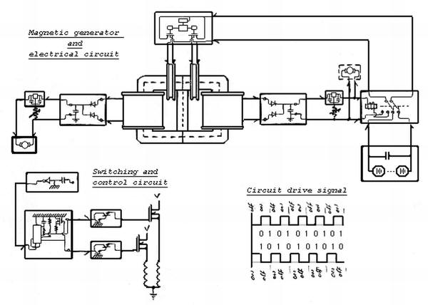
The MEG Simulations:
The
Basic architecture of the MEG, Magnet Placement and Actuator
coil alignment and pole directions.
Graphed
Input to the Actuator Coils:
Animation
slowed down so it is visible what's is happening in The
MEG

For
more detailed information please read on.
|
|
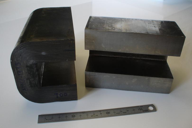
The
Core - Metglas® Alloy 2605SA1:
| |
|
|
| |
|
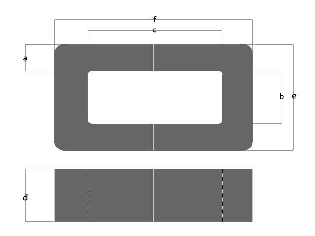
CORE # |
AMCC-1775 |
a
(mm) |
33.0±1.0 |
b
(mm) |
40.5±0.5 |
c
(mm) |
106.30±1.25 |
d
(mm) |
142.00±1.5 |
e*
(mm) |
106.5±2.5 |
f*
(mm) |
172.6+4.0 |
Lm*
(cm) |
39.72 |
Ac*
(cm2) |
39.36 |
Core
Wt.±2%
(gm) |
11466.0 |
Window
Area
(cm2)
|
43.05 |
|
 |
|
The material,
known as Metglas, was commercialized in early 1980s and
used for low-loss power distribution transformers (Amorphous
metal transformer). Metglas-2605 is composed of 80% iron
and 20% boron, has Curie temperature of 373 °C and a room
temperature saturation magnetization of 125.7 milliteslas.
An amorphous metal is a metallic material with a disordered
atomic-scale structure. In contrast to most metals, which
are crystalline and therefore have a highly ordered arrangement
of atoms, amorphous alloys are non-crystalline. Materials
in which such a disordered structure is produced directly
from the liquid state during cooling are called "glasses",
and so amorphous metals are commonly referred to as "metallic
glasses" or "glassy metals". However, there are several
other ways in which amorphous metals can be produced, including
physical vapor deposition, solid-state reaction, ion irradiation,
melt spinning, and mechanical alloying. Amorphous metals
produced by these techniques are, strictly speaking, not
glasses. However, materials scientists commonly consider
amorphous alloys to be a single class of materials, regardless
of how they are prepared.
In the past, small batches of amorphous metals have been
produced through a variety of quick-cooling methods. For
instance, amorphous metal wires have been produced by sputtering
molten metal onto a spinning metal disk. The rapid cooling,
on the order of millions of degrees a second, is too fast
for crystals to form and the material is "locked in" a glassy
state. More recently a number of alloys with critical cooling
rates low enough to allow formation of amorphous structure
in thick layers (over 1 millimeter) had been produced, these
are known as bulk metallic glasses (BMG). Liquidmetal sells
a number of titanium-based BMGs, developed in studies originally
carried out at Caltech. More recently, batches of amorphous
steel have been produced that demonstrate strengths much
greater than conventional steel alloys.
The alloys
of
boron,
silicon,
phosphorus, and other glass formers with magnetic metals
(iron,
cobalt,
nickel) are magnetic, with low
coercivity and high
electrical resistance. The high resistance leads to
low losses by
eddy currents when subjected to alternating magnetic
fields, a property useful for eg.
transformer
magnetic cores.
Ref:
http://en.wikipedia.org/wiki/Amorphous_metal
|
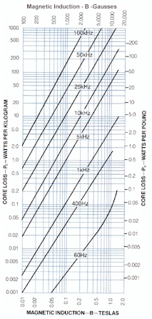
Typical Impedance
Permeability Curves & Typical Core Loss Curves:
|
| |
|
General Properties & Characteristics
|
|
ELECTROMAGNETIC |
|
|
Saturation Induction (T) |
|
As Cast
|
1.56 |
|
Maximum DC Permeability (µ):
|
Annealed (High Freq.)
|
600,000 |
As Cast
|
45,000 |
|
Saturation Magnetostriction (ppm) |
27 |
|
Electrical Resistivity (µ-cm) |
130 |
|
Curie Temperature (°C) |
399 |
|
|
|
PHYSICAL |
|
Thickness (mils) |
1.0 |
|
Standard Available Widths |
|
|
Minimum (inches)
|
0.2 |
|
Maximum (inches)
|
8.4 |
|
Density (g/m3) |
|
As Cast
|
7.18 |
|
Vicker's Hardness (50g Load) |
900 |
|
Tensile Strength (GPa) |
1-2 |
|
Elastic Modulus (GPa) |
100-110 |
|
Lamination Factor (%) |
>79 |
|
Thermal Expansion (ppm/°C) |
7.6 |
|
Crystallization Temperature (°C) |
508 |
|
Continuous Service Temp. (°C) |
150 |
|
|
|
|
|
B H Curve:

|
|
|
I got my cores
from http://www.uaml.net/.
The Contact there is Vikas. He is very helpful. Please mention
Chris from hyiq.org and Vikas will help you out.
|
|
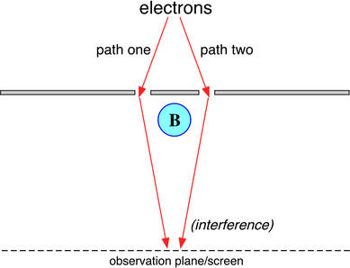
Aharonov-Bohm
Effect:
|
Magnetic Aharonov–Bohm effect
The magnetic Aharonov–Bohm
effect can be seen as a
result of the requirement
that quantum physics be
invariant with respect to
the
gauge choice for the
vector potential A.
This implies that a particle
with electric charge
q travelling along some
path P in a region with
zero magnetic field ( )
must acquire a phase )
must acquire a phase
 ,
given in
SI units by ,
given in
SI units by
-
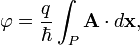
with a phase difference
 between any two paths with
the same endpoints therefore
determined by the
magnetic flux Φ through
the area between the paths
(via
Stokes' theorem and
between any two paths with
the same endpoints therefore
determined by the
magnetic flux Φ through
the area between the paths
(via
Stokes' theorem and
 ),
and given by: ),
and given by:
-

-
This phase difference can
be observed by placing a
solenoid between the
slits of a double-slit experiment
(or equivalent). An ideal
solenoid encloses a magnetic
field B, but does
not produce any magnetic
field outside of its cylinder,
and thus the charged particle
(e.g. an
electron) passing outside
experiences no classical
effect. However, there is
a (curl-free)
vector potential outside
the solenoid with an enclosed
flux, and so the relative
phase of particles passing
through one slit or the
other is altered by whether
the solenoid current is
turned on or off. This corresponds
to an observable shift of
the interference fringes
on the observation plane.
The same phase effect is
responsible for the
quantized-flux requirement
in
superconducting loops.
This quantization is because
the superconducting wave
function must be single
valued: its phase difference
Δφ around a closed loop
must be an integer multiple
of 2π (with the charge
q=2e for the
electron Cooper pairs),
and thus the flux Φ must
be a multiple of h/2e.
The superconducting flux
quantum was actually predicted
prior to Aharonov and Bohm,
by London (1948)
using a phenomenological
model.
The magnetic Aharonov–Bohm
effect is also closely related
to
Dirac's argument that
the existence of a
magnetic monopole necessarily
implies that both electric
and magnetic charges are
quantized. A magnetic monopole
implies a mathematical singularity
in the vector potential,
which can be expressed as
an infinitely long
Dirac string of infinitesimal
diameter that contains the
equivalent of all of the
4πg flux from a monopole
"charge" g. Thus,
assuming the absence of
an infinite-range scattering
effect by this arbitrary
choice of singularity, the
requirement of single-valued
wave functions (as above)
necessitates charge-quantization:
 must be an integer (in
cgs units) for any electric
charge q and magnetic
charge g.
must be an integer (in
cgs units) for any electric
charge q and magnetic
charge g.
The magnetic Aharonov–Bohm
effect was experimentally
confirmed by Osakabe et
al. (1986), following much
earlier work summarized
in Olariu and Popèscu (1984).
Its scope and application
continues to expand. Webb
et al. (1985) demonstrated
Aharonov–Bohm oscillations
in ordinary, non-superconducting
metallic rings; for a discussion,
see Schwarzschild (1986)
and Imry & Webb (1989).
Bachtold et al. (1999) detected
the effect in carbon nanotubes;
for a discussion, see Kong
et al. (2004).
Electric Aharonov–Bohm effect
Just as the phase of the
wave function depends upon
the magnetic vector potential,
it also depends upon the
scalar electric potential.
By constructing a situation
in which the electrostatic
potential varies for two
paths of a particle, through
regions of zero electric
field, an observable Aharonov–Bohm
interference phenomenon
from the phase shift has
been predicted; again, the
absence of an electric field
means that, classically,
there would be no effect.
From the
Schrödinger equation,
the phase of an eigenfunction
with energy E goes
as
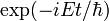 .
The energy, however, will
depend upon the electrostatic
potential V for a
particle with charge
q. In particular, for
a region with constant potential
V (zero field), the
electric potential energy
qV is simply added
to E, resulting in
a phase shift: .
The energy, however, will
depend upon the electrostatic
potential V for a
particle with charge
q. In particular, for
a region with constant potential
V (zero field), the
electric potential energy
qV is simply added
to E, resulting in
a phase shift:
-
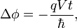
where t is the time
spent in the potential.
The initial theoretical
proposal for this effect
suggested an experiment
where charges pass through
conducting cylinders along
two paths, which shield
the particles from external
electric fields in the regions
where they travel, but still
allow a varying potential
to be applied by charging
the cylinders. This proved
difficult to realize, however.
Instead, a different experiment
was proposed involving a
ring geometry interrupted
by tunnel barriers, with
a bias voltage V
relating the potentials
of the two halves of the
ring. This situation results
in an Aharonov–Bohm phase
shift as above, and was
observed experimentally
in 1998.
Ref: http://en.wikipedia.org/wiki/Aharonov-Bohm_effect
|
|
|
|
|